Dynamic Programming in Haskell

 

For my next little project, I decided to try to implement a dynamic programming solution for the Longest Common Subsequence (LCS) problem.

I learned about dynamic programming in university, but I had a lot of trouble understanding exactly how it works. Attempting to program a dynamic programming algorithm in Haskell has helped me understand the fundamental principles behind dynamic programming in a way that I wasn’t able to when I learned it from an imperative programming perspective.

What is Dynamic Programming?

In dynamic programming, you have a problem where your goal is to find the optimal value of a function F on a particular input, where F has two properties:

• Optimal sub-structure. This means that for F can be broken into multiple sub-problems, each of which has an optimal solution and the optimal solution for F is a combination of the optimal solutions to the sub-problems of F. In general, the sub-problems of F have sub-problems themselves, so dynamic programming is a naturally recursive kind of problem.
• Overlapping sub-problems. This means that while you recursively evaluate the optimal solution for F, you evaluate some of its recursive sub-problems more than once. Since there is only one optimal solution to each sub-problem (because the sub-problem functions are pure functions, and are referentially transparent), you are wasting time evaluating the repeated sub-problems over and over again if you re-evaluate their sub-problems. Instead, you want to memoize the sub-problems by storing them in some kind of cache so you don’t have to re-compute them.

In the case of the LCS problem, we want to compute the longest sub-sequence of characters between two strings (we could do this on two sequences of any type, but strings are used as a common example). It turns out that this problem has optimal substructure and overlapping sub-problems, and so we can use dynamic programming to solve it efficiently.

When this was taught to me in university, the emphasis was on the implementation of a solution using a matrix, rather than on the principle of dynamic programming which can be applied in the case of any problem with both optimal substructure and overlapping sub-problems.

The principle is that for any problem, F(i, j), there are sub-problems F(i – 1, k), where

F(i, j) = G(F(i – 1, 0), F(i – 1, 1), …)

In other words, you need to know the optimal solutions of the sub-problems F(i – 1, k) and you apply a function G to the values of the sub-problems to compute F(i, j).

In addition, since the sub-problems overlap, the values of the sub-problems F(i – 1, k) are stored in some kind of cache, perhaps a list, graph, hash table, or in the case of LCS, a matrix. This allows you to avoid re-computing sub-problem values which you have computed previously.

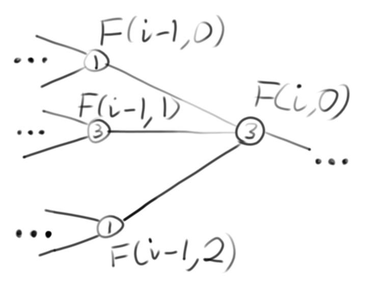
The LCS problem, and every other dynamic programming problem, can be visualized as a graph problem, where each problem is a vertex and each sub-problem is connected to its parent problem with an edge:

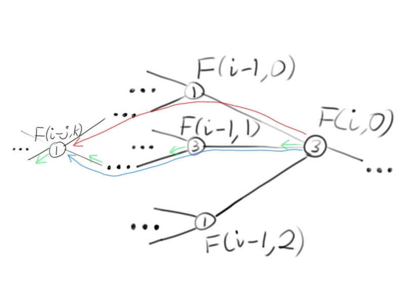
In order to memoize a general dynamic programming problem, you can cache the optimal solution for each sub-problem at each vertex as meta-data. A problem has overlapping sub-problems if there are two paths to reach the same sub-problem, F(i – j, k), from the problem, (F(i, 0)):

Instead of re-computing the overlapping sub-problem, F(i – j, k), when you encounter it the second time, you can access the cached value to avoid re-computing it.

Sometimes, you may need to recover the path taken for the optimal solution, you can store which edge to take to get to the best sub-problem. When you can choose an edge to take which represents the optimal solution, the dynamic programming problem is called a dynamic decision problem. (The little arrows next to each node represent the edge chosen for the optimal sub-problem).

This method of storing which edges represent the optimal solution is used in the LCS computation.

F(i, 0) can then be computed using the cached values with the function you saw above:

F(i, 0) = G(F(i – 1, 0), F(i – 1, 1), F(i – 1, 2))

In the case of the longest common sub-sequence, the function G is called LCS and is defined like this:

For two strings A and B of length m and n  respectively, the LCS of those strings is:

LCS(A[0, m], B[0, n])
    | A[m - 1] == B[n - 1] = 1 + LCS(A[0, m - 1], B[0, n - 1])
    | otherwise = max(LCS(A[0, m - 1], B[0, n]), LCS(A[0, m], B[0, n - 1])

Here we are computing the length of the LCS of A and B. Whenever the length of the LCS increases by 1, we have added a character to the LCS which matches in A and B.

As you can see, the problem is solved by computing optimal solutions to LCS on prefixes of A and B. In order to get a prefix of A or B which is one smaller than A or B, we remove one character from either A or B. The LCS of the first character of A and B is 0 if A[0] != B[0] and 1 if A[0] == B[0]. This is our terminal case for the recursion.

In the general case, to find the LCS of A and B, there are two cases, either the last character of A and B are the same, or they differ.

Let’s give the name P to the last character of A and Q to the last character of B. if P and Q are the same, the P must be a part of the LCS of A and B because P is common to A and B and any sub-sequence which doesn’t include P would be shorter than a sequence which ends with P. The LCS of A and B must be whatever the LCS of A and B are with P removed, plus P.

In the case where P and Q differ, they can not be in the LCS of A and B because they are not common to both A and B. In this case, it is possible that the LCS of A and B is the LCS of A with P removed and B or the LCS of A and B with Q removed. In order to compute an optimal LCS, we must choose whichever is longer.

You may be tempted to ask “aren’t we forgetting about the case P is not equal to Q and where we remove both P from A and Q from B?”; let’s call this case the “overlapping sub-problem”. You could include a check for the overlapping sub-problem too, but it would be a waste of time, because it is an overlapping sub-problem of both LCS(A[0, m – 1], B[0, n]), and LCS(A[0, m], B[0, n – 1]). In the first case, we can remove Q from B to form the overlapping sub-problem and in the second case we can remove P from A to form the overlapping sub-problem. Since the overlapping sub-problem is a sub-problem of a sub-problem, we don’t need to write a special case for it in the recursion because it will naturally be handled by recursively applying the first two cases.

It is important to note that up until this point, we have only been computing the length of the LCS, which is not the goal of this algorithm, which is to find the sub-sequence itself. In order to compute the sub-sequence, we should note that when the LCS increases in length, a character is added to the LCS, and when it doesn’t increase in length, we are choosing which sub-problem contains the longer common sub-sequence. In order to find the LCS, of two strings A and B, we should add the last character P/Q to the LCS if LCS(A, B) is greater than LCS(A[0, m – 1], B[0, n – 1]) and if not, we should choose to consider a prefix of A and B based on which of LCS(A[0, m – 1], B) and LCS(A, B[0, n – 1]) is larger.

 

In practice, we can efficiently compute the LCS using a matrix for memoization:

Using a matrix allows us to access the cache in constant time. Notice that an extra empty character has been prefixed to both strings, so that the terminating condition of the LCS function when the length of the sub-string is 0 is length 0. If the ith entry in A is equal to the jth entry in B, then we only need to access the cached value in F(i – 1, j – 1), otherwise we need to take the maximum value of F(i – 1, j) and F(i, j – 1).

Code Time

Let’s examine how to implement this in Haskell.

Firstly, we need to use the Data.Array and Data.Matrix packages for constant time access to the cache and strings:

import Data.Array ((!)) --Import the array index operator
import qualified Data.Array
import qualified Data.Matrix

Since we want to recover the path taken for the decision problem, we also need a direction to travel in the matrix using a Direction type:

data Direction = NoDir | LeftDir | UpDir | DiagonalDir deriving (Show, Eq)

The main function takes two strings, converts them into arrays, and calls lcs on them:

main = getArgs >>= (\args ->
       case args of
       [] -> putStrLn "Please enter two strings for lcs"
       (a : []) -> putStrLn "Please enter two strings for lcs"
       (a : b : []) -> let arrayA = Data.Array.listArray (0, length a) a
                           arrayB = Data.Array.listArray (0, length b) b
                       in lcs arrayA arrayB (initMatrix (length arrayA) (length arrayB)))

The two strings are called a and b.

initMatrix just sets up a matrix with all zero entries and no direction:

initMatrix :: Int -> Int -> Data.Matrix.Matrix (Direction, Int)
initMatrix a b = Data.Matrix.matrix a b (\(i, j) -> (NoDir, 0))

lcs is broken into two parts, first the sub-problem matrix is computed in lcsMatrix and then the optimal path is traced through the matrix in traceMatrix. lcs prints out the resulting longest common sub-sequence:

lcs :: Data.Array.Array Int Char -> Data.Array.Array Int Char -> Data.Matrix.Matrix (Direction, Int) -> IO ()
lcs a b m = putStrLn (traceMatrix (length a - 1) (length b - 1) a b subProblemMatrix "")
              where subProblemMatrix = lcsMatrix (length a - 1) (length b - 1) a b m

Note that lcsMatrix and traceMatrix both start at the bottom right corner of the matrix and recursively traverse towards the top left.

lcsMatrix updates the matrix cache with the value of the LCS for the coordinates i and j:

lcsMatrix :: Int -> Int -> Data.Array.Array Int Char -> Data.Array.Array Int Char -> Data.Matrix.Matrix (Direction, Int) -> Data.Matrix.Matrix (Direction, Int)
lcsMatrix 0 0 _ _ m = m
lcsMatrix 0 _ _ _ m = m
lcsMatrix _ 0 _ _ m = m
lcsMatrix i j a b m = let (thisDir, thisValue) = Data.Matrix.getElem (i + 1) (j + 1) m
                      in updateMatrix thisDir i j a b m

Annoyingly, Data.Matrix is 1-indexed instead of 0-indexed, so we need to add 1 to each coordinate; instead of (i, j) we need to use (i + 1, j + 1).

lcsMatrix terminates without updating the cache whenever it reaches the top or left of the matrix.

updateMatrix performs the actual memoized evaluation of the LCS function I defined above:

updateMatrix :: Direction -> Int -> Int -> Data.Array.Array Int Char -> Data.Array.Array Int Char -> Data.Matrix.Matrix (Direction, Int) -> Data.Matrix.Matrix (Direction, Int)
updateMatrix NoDir i j a b m
 | (a ! (i - 1)) == (b ! (j - 1))
      = let diagM = lcsMatrix (i - 1) (j - 1) a b m
            (diagDir, diagValue) = Data.Matrix.getElem i j diagM
        in Data.Matrix.setElem (DiagonalDir, (1 + diagValue)) (i + 1, j + 1) diagM
 | otherwise = let leftM = lcsMatrix (i - 1) j a b m
                   upM = lcsMatrix i (j - 1) a b leftM
                   (leftDir, leftValue) = Data.Matrix.getElem (i + 1) j upM
                   (upDir, upValue) = Data.Matrix.getElem i (j + 1) upM
               in if leftValue < upValue
               then Data.Matrix.setElem (UpDir, upValue) (i + 1, j + 1) upM
               else Data.Matrix.setElem (LeftDir, leftValue) (i + 1, j + 1) upM
updateMatrix _ _ _ _ _ m = m --Matrix already has a value here

! is the array indexing operator.

There are a few cases to consider here.

First, the second pattern is matched if direction is anything other than NoDir. This means that if you call updateMatrix on any element which has a direction, the cache is used instead of computing the matrix update. Pattern matching makes it pretty simple to implement memoization in Haskell.

In the other pattern, the expression (a ! (i – 1)) == (b ! (j – 1)) tests if the character at the i and j locations in the strings are equal. The reason we have to subtract 1 here is because an empty character was prefixed onto the strings in the matrix, so the matrix index is off-by-one relative to the string index.

In the case where the characters are equal,  we need to consider the diagonal element, which is computed like this:

diagM = lcsMatrix (i - 1) (j - 1) a b m

The cache is implicitly checked and updated by lcsMatrix, so we need to use the matrix returned by the function for all future queries. Next, we want the diagonal element (i – 1, j – 1):

(diagDir, diagValue) = Data.Matrix.getElem i j diagM

Then we can update the matrix element at (i, j) with 1 + the diagonal value:

Data.Matrix.setElem (DiagonalDir, (1 + diagValue)) (i + 1, j + 1) diagM

Again, since we want to set the element (i, j) in Data.Matrix, we need to add 1 to each coordinate to get (i + 1, j + 1). Notice that I stored a DiagonalDir in the Matrix, this will be used later to trace the LCS.

In the case where the two characters don’t match, we need to get the left and up neighbor values. These are computed or retrieved from the cache using the lcsMatrix function:

leftM = lcsMatrix (i - 1) j a b m
upM = lcsMatrix i (j - 1) a b leftM

Notice that I am passing leftM as a parameter to the up neighbor computation. This is because the up neighbor computation may benefit from the cache updates computed in the left neighbor computation. In general, you need to use the latest version of your state wherever possible.

Once we’ve updated the matrix caches, we can read from the updated matrices:

(leftDir, leftValue) = Data.Matrix.getElem (i + 1) j upM
(upDir, upValue) = Data.Matrix.getElem i (j + 1) upM

The LCS function chooses the maximum LCS value from each of these and updates the matrix appropriately:

if leftValue < upValue
then Data.Matrix.setElem (UpDir, upValue) (i + 1, j + 1) upM
else Data.Matrix.setElem (LeftDir, leftValue) (i + 1, j + 1) upM

Notice that I have stored UpDir and LeftDir in the matrix to use for tracing the LCS in traceMatrix.

All that remains is to trace the LCS starting at the final element:

traceMatrix :: Int -> Int -> Data.Array.Array Int Char -> Data.Array.Array Int Char -> Data.Matrix.Matrix (Direction, Int) -> [Char] -> [Char]
traceMatrix i 1 a b _ longestCommonSubsequence
    | a ! (i - 1) == b ! 0 = (a ! (i - 1)) : longestCommonSubsequence
    | otherwise = longestCommonSubsequence
traceMatrix 1 j a b _ longestCommonSubsequence
    | a ! 0 == b ! (j - 1) = (a ! 0) : longestCommonSubsequence
    | otherwise = longestCommonSubsequence
traceMatrix i j a b m longestCommonSubsequence
    = let (direction, _) = Data.Matrix.getElem (i + 1) (j + 1) m
      in case direction of
         LeftDir -> traceMatrix i (j - 1) a b m longestCommonSubsequence
         UpDir -> traceMatrix (i - 1) j a b m longestCommonSubsequence
         DiagonalDir -> traceMatrix (i - 1) (j - 1) a b m (a ! (i - 1) : longestCommonSubsequence)

The first and second patterns match the cases when either i or j is 1. In the case where the characters match, they are added to the longestCommonSubsequence, otherwise the function evaluates to the existing sub-sequence. These are the terminal cases for the recursion.

The third pattern matches the general case of the recursion for element (i, j). The first thing which happens is the direction is extracted from the matrix for the element:

(direction, _) = Data.Matrix.getElem (i + 1) (j + 1) m

In the case where the direction is LeftDir or UpDir, the recursion just continues with the left neighbor’s index or up neighbor’s index respectively:

LeftDir -> traceMatrix i (j - 1) a b m longestCommonSubsequence
UpDir -> traceMatrix (i - 1) j a b m longestCommonSubsequence

In the case where the direction is DiagonalDir, that means that we discovered an element of the LCS in lcsMatrix, the current character is added to the longestCommonSubsequence and the recursion contiues with the diagonal neighbor’s index:

DiagonalDir -> traceMatrix (i - 1) (j - 1) a b m (a ! (i - 1) : longestCommonSubsequence)

Altogether, these operations will compute the LCS of a and b.

The code for this post can be found here: https://github.com/WhatTheFunctional/LCS